How to do Programming

TL;DR: Identify assumptions and write them down.

There’s a common (I think) misconception that the programming trade is all about knowing obscure facts and doing hard math. From this it follows that a person has to get really good at math or know a huge number of things before doing programming.

Unfortunately people who have this misconception can be discouraged from trying in the first place. It might be unrealistic to think that every single person not only can but also will want to do it, but I think that lots of people with this misconception could do very well at programming, once they understand what it is actually like, and if they put some effort into learning it.

In reality, being good at the math or knowing all about compilers and language features does not help with a large percentage of the day-to-day work that most programmers do. Instead, their effort goes into writing down all the assumptions made by the high-level description of a feature. In other words, the requirements will say “display a count of the current total” and the programming work is about finding the assumptions implied by that description (“what does ‘current’ actually mean?” etc), then writing them down explicitly. Once you write down the assumptions in the right way, the explicit representation of the assumptions is your code and you are done. Getting everything written down correctly used to be much harder, but with modern programming tools it isn’t even possible to make some of the most problematic mistakes anymore, and the tools can catch lots of other mistakes automatically. For everything else you would want to get help from a more experienced colleague, or just ask strangers on Stack Overflow.

There are programmers who would take issue with this description. I’m using the terms “doing programming” and “day-to-day programming” strategically, really to mean commercial or hobbyist programming for which there are mature high-quality tools and well-understood best practices. On the cutting edge of academia, and within programming projects that have very demanding requirements, advanced math and knowing lots of obscure facts can be much more important.

Basically, what I’m saying is that people tend to confuse the larger industry with that super-difficult hacker nerd work they see in movies and TV shows. In fact, the vast majority of programming work going on right now is the other kind. There are huge numbers of those jobs to be done, because it is where all the theory and advanced knowledge finally can be applied to a real-world problem. Many large software teams have so much of this kind of work that they split out a whole department for “requirements engineering”, which is taking the really high-level descriptions with tons of assumptions, and breaking those out into statements with fewer or no assumptions left in each statement, so that the code writers can focus on making the final code work. The best requirements are harder to write than all the coding work that comes after!

Maybe someone has told you before that programming is all about breaking problems down into smaller problems. It’s another way of saying the same thing.


Fractals

Last time we plotted a Mandelbrot set using a small Python script. This set is interesting because an unexpectedly large amount of detail emerges from the iteration of a relatively simple function. Even more interesting is the fact that this detail is not limited to any particular resolution. The Mandelbrot set exhibits fractal geometry, meaning that tiny areas of the set share features with the whole thing. If we zoom in, smaller details are visible no matter how far we choose to zoom.

But you don’t have to believe me – let’s modify our Python script and see what happens. Basically we have to map 600 pixels in each direction to arbitrary sections of the real and imaginary axes. We can have our script read in the desired ranges and calculate appropriate mappings. First, store the inputs in decimal variables:

def get_decimal(m):
    while True:
        try:
            x = float(input(m))
            return x
        except ValueError:
            print('Enter a decimal number.')

loX = get_decimal('Minimum X: ')
hiX = get_decimal('Maximum X: ')
loY = get_decimal('Minimum Y: ')
hiY = get_decimal('Maximum Y: ')

Divide 600 by the range in each direction to compute scale coefficients:

scaleX = 600.0/(hiX - loX)
scaleY = 600.0/(hiY - loY)

Now modify the drawing code to use our designated ranges:

for x in range(0,600):
    real = loX + x / scaleX
    for y in range(0, 600):
        imag = loY + y / scaleY
        c = complex(real, imag)
        p = mandel(c)
        w.create_line(x, 600-y, x+1, 601-y, fill=colors[p])
        w.pack()

With these changes we can zoom in and see some interesting features. Try using -0.15, -0.05, 0.9, and 1.0 as input values. More detail is visible, but it looks like some of the boundaries are smoothing out! Interestingly, that’s because our mandel() function only checks whether each candidate c escapes within 20 iterations. Points close to the boundary often take more than 20 iterations to escape, but they don’t actually belong in the set. Therefore, as the zoom level increases we have to test each candidate c for more iterations in order to maintain an accurate image. This is left as an exercise for the reader.

The Mandelbrot Set

Last year we considered complex numbers, quantities with two degrees of freedom. These numbers have many important applications in engineering, but can we immediately use them to do something interesting?

Well, we can draw the Mandelbrot set with a computer and a bit of ingenuity. This set includes every complex number for which the following recurrence equation never produces a result with an absolute value (distance from the complex origin) greater than two:

mandelbrotequation

For any complex number, we start with z = 0, square it, add our complex candidate c, then repeat the process with z equal to the new (complex) value. As long as z stays close to the origin after many iterations, our candidate is probably in the Mandelbrot set. Since complex numbers behave like points in a 2D plane, we can draw an image where each pixel is colored by testing a candidate c related to its horizontal and vertical position.

So let’s make a drawing! This program is based on Prez Jordan’s Python code, but we’ll add a gradient to show how many iterations each candidate takes to escape. First we set up a 600×600 canvas with Tkinter:

from Tkinter import Tk, Canvas, mainloop

tk = Tk()
w = Canvas(tk, width=600, height=600)

Next we define our mandel() function which takes a complex number and tests whether it escapes in twenty iterations. If so the function returns the last iteration number, otherwise it returns 99:

def mandel(c):
    z = 0
    i = 0
    for h in range(0,20):
        z = z*z + c
        if abs(z) > 2:
            break
        else:
            i+=1
    if abs(z) >= 2:
        return i
    else:
        return 99

In order to draw a gradient, let’s use a dictionary to map iterations to colors. We’ll need entries for keys 0-20 and 99:

colors = {
    0: 'white',
    1: 'white',
    2: 'light yellow',
    3: 'light yellow',
    4: 'lemon chiffon',
    5: 'lemon chiffon',
    6: 'yellow',
    7: 'yellow',
    8: 'gold',
    9: 'gold',
    10: 'orange',
    11: 'orange',
    12: 'orange red',
    13: 'orange red',
    14: 'red',
    15: 'red',
    16: 'red',
    17: 'dark red',
    18: 'dark red',
    19: 'dark red',
    20: 'dark red',
    99: 'black'
}

Finally we loop over each pixel, convert its x and y coordinates to a complex number, test that number by passing it to the mandel() function, and use the returned key to look up the appropriate color in our dictionary:

print "Drawing..."

for x in range(0,600):
    real = x / 200.0 - 2.2
    for y in range(0, 600):
        imag = y / 200.0 - 1.5
        c = complex(real, imag)
        p = mandel(c)
        w.create_line(x, 600-y, x+1, 601-y, fill=colors[p])
        w.pack()

print "Complete!"
mainloop()

Run this code in your Python interpreter and see a picture of the Mandelbrot set!

Falsifiability

According to Karl Popper, any scientific theory must be falsifiable. What does this entail?

A falsifiable theory leads to predictions which would be invalidated by some conceivable observation. For example, Newtonian dynamics predicts that in a uniform gravitational field, two objects with different masses will have the same acceleration due to gravity. It implies that if we drop a feather and a ball bearing inside a vacuum chamber, the ball bearing will not fall faster, as long as the theory is valid. This is in fact what happens.

Newton’s theory was very successful at describing the celestial motion of the known planets, but in the 19th century it did not correctly predict the orbit of Uranus. This fact would have falsified the theory, or greatly limited its precision. However, Urbain Le Verrier knew that the gravitational field of an unknown planet could be pulling Uranus into its observed orbit, and predicted where and how massive such a planet would be. Astronomers pointed their telescopes at the expected location and discovered Neptune. If no planet had existed at that location, this prediction would have been wrong, and the inconsistency with Newtonian dynamics would have remained valid.

A planet orbits in an ellipse, and the point where it moves closest to the sun is called the perihelion of its orbit. This point gradually precesses around the sun due to gravitational forces exerted by other planets. The same Le Verrier compared observations of Mercury to the perihelion precession rate derived from Newton’s theory, and found a discrepancy of nearly half an arcsecond per year. He predicted the existence of another planet closer to the sun to explain his result, but no planet was ever observed and this problem remained open.

To explain other puzzling observations, Albert Einstein abandoned the Galilean transformations of Newton’s theory for a framework which uses Lorentz transformations in four dimensions. General Relativity describes gravitation as an effect of spacetime curvature. It simplifies to Newtonian dynamics at lower energy levels. According to this theory, the perihelion of Mercury’s orbit should precess by an additional 0.43 arcseconds per year, matching the observed value.

Still, the intuitive simplicity of Einstein’s theory did not automatically mean that it was a valid replacement for Newtonian dynamics. During the total solar eclipse of 1919, measured deflection of starlight agreed with the value derived from General Relativity, a highly publicized result. Decades passed before additional predictions were conclusively validated.

Degrees and Freedom

Here’s my idea of a good math lesson. I want to explain Euler’s formula, the cornerstone of multidimensional mathematics, and one of the truly beautiful ideas from history. In school this formula appears as a useful trick, and is not commonly understood. I think that is because students are denied enough time to wonder what the formula actually means (it doesn’t describe how to pass an exam). Here is Euler’s formula:

e^(ix) = cos(x) + i*sin(x)

This idea was introduced to me after a review of imaginary and complex numbers. Once the history and definition were out of the way, we completely freaked out at the idea of putting ‘i’ in the exponent, then practiced how to use it in calculations. I might have had a brief moment of clarity in that first class, but by the AP exam Euler’s formula was nothing more than a black box for converting rectangular coordinates to polar coordinates.

Many years later, I came across the introduction to complex numbers from Feynman’s Lectures on Physics, and suddenly the whole concept clicked in a way that it never had in school. Explained here, I don’t think it is really that difficult to understand, but then I’ve already managed to understand it, so I’ll try to communicate my understanding and then you can tell me whether it makes sense.

We need to start by generalizing the concept of a numeric parameter. The number line from grade school is an obvious way to represent a system with one numeric parameter. If we label the integers along this line, each mark corresponds to a grouping of whole, countable things, and the value of our integer parameter must refer to one of these marks. If we imagine a similar system where our parameter can “slide” continuously from one integer to the next, the values that we can represent are now uncountable (start counting the numbers between 0.001 and 0.002 if you don’t believe me) but opening up this unlimited number of in-between values allows us to model continuous systems that are much harder to represent with chunks.

Each system has a single numeric parameter, even though the continuous floating-point parameter can represent numbers that the integer parameter cannot. In physics, the continuous parameter can represent what is called a “degree of freedom,” basically a quantity that changes independently of every other quantity describing the system. Sometimes a “degree of freedom” is just like one of the three dimensions that you can see right… now, but this is not always the case. Wavefunctions in particle physics can have infinite degrees of freedom, even though the objects described by these esoteric equations follow different laws when we limit our models to the four parameters of spacetime.

Anyway, the imaginary unit or ‘i’ is just some different unit that identifies a second numeric parameter. If we multiply an integer by ‘i’, we’re basically moving a second parameter along its own number line that same distance. Apply the “sliding” logic from before and we can use the fractional parts between each imaginary interval. If this sounds new and confusing, just remember that any “real” number is itself multiplied by the real unit, 1. Personally, I don’t think that the word “imaginary” should be used to describe any kind of number, because all numbers are obviously imaginary. However, this convention exists regardless of how I feel about it, and nobody would know what to put in Google if I used a different word.

Why do teachers use this system where one implicit unit is supplemented by a second explicit unit? Simple – it was added long before anyone fully understood what was going on. The imaginary unit was the invented answer to a question, that question being:

Which number yields -1 when multiplied by itself?

The first people to ask this question didn’t get much further than “A number called ‘i’ which is nowhere on the number line, and therefore imaginary.” If those scholars had described their problem and its solution in a different way, they might have realized some important things. First, this question starts with the multiplicative identity (1) and really asks “which number can we multiply 1 by twice, leaving -1?” Thinking about it like this, it soon becomes clear that the range of values we can leave behind after multiplying 1 by another value on the same number line, twice, cannot include -1! We can make 1 bigger, twice, by multiplying it by a larger integer, or smaller, by multiplying it by a value between 0 and 1. We can also negate 1 twice while scaling it up or down, but none of these options allow for a negative result!

A clever student might point out that this is a stupid answer and that we might as well say there is none, but we still learn about it because amazing things happen if we assume that some kind of ‘i’ exists. We can imagine a horizontal number line, and then a second number line going straight up at 90° (τ/4 radians, a quarter turn) from the first. Moving a point along one line won’t affect its value on the other line, so we can say that the value of our ‘i’ parameter is represented on the vertical line and the value of our first (“real”) parameter is represented on the horizontal line. That is, a complex number (a*1+b*i) imagined as a single point on a 2-dimensional plane. In this space, purely “real” or purely “imaginary” numbers behave just like complex numbers with zero for the value of one parameter.

Now think about the answer to that question again. If our candidate is ‘i’ or some value up “above” the real number line, it’s easy to imagine a vector transformation (which we assume still works like multiplication) that can change 1 to ‘i’ and then ‘i’ to -1 in this 2D number space. Just rotate the point around the origin by 90°. When our parameters are independent like this, exponentiation by some number of ‘i’ units is exactly like rotating the imagined “point” a quarter turn around zero some number of times. I don’t really know why it works, but it works perfectly!

We’ve seen that imaginary units simply measure a second parameter, and how this intuitively meshes with plane geometry. Now let’s review what is actually going on. Numbers multiplied by ‘i’ behave almost exactly like numbers multiplied by 1, but the important thing about all ‘i’ numbers is that they are different from all non-‘i’ numbers and therefore can’t be meaningfully added into them. The ‘i’ parameter is a free parameter in the two-parameter system that is every complex number. It can get bigger or smaller without affecting the other parameter.

Bringing this all together, let’s try to understand what Euler was thinking when he wrote down his formula, and why it was such a smashing success. He noticed that the Taylor series definition of the exponential function:

Exponential function and its Taylor series

Becomes this:
Complex exponential and its Taylor series

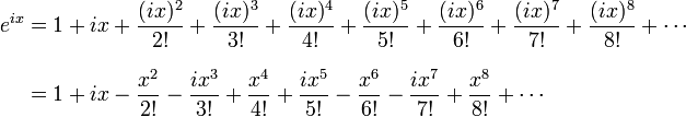
When ‘i*x’ is the exponent, because the integer powers of ‘i’ go round our complex circle from 1 to i to -1 to -i and back. Grouping the real terms and the ‘i’ terms together suddenly and unexpectedly reveals perfect Taylor series expansions of the cosine and sine:
Euler's complex exponential series

As each expansion is multiplied by a different free parameter, the two expansions don’t add together, naturally separating the right side of our equation into circular functions! We can just conclude that those functions really are the cosine and sine of our variable, remembering that the sine is an ‘i’ parameter, and it works! Because these expressions are equivalent, having a variable in the exponent allows us to multiply our real base by ‘i’ any fractional number of times (review your exponentials), and thus rotate to any point in the imagined complex plane. There are other ways to prove this formula, but I still do not understand exactly why any of the proofs happen the way they do. It’s not really a problem, because Euler probably didn’t understand it either, but I’d still like to come across a good answer someday. What I know right now is that any complex number can be encoded as a real number rotated around zero by an imaginary exponent:

e^(ix) = cos(x) + i*sin(x)

Here is proof that certain systems of two variables can be represented by other systems of one complex variable in a different form, and the math still works! Euler’s formula is a monumental, paradigm-shattering shortcut, and it made the modern world possible. I’m not overstating that point at all, everything from your TV to the Mars rover takes advantage of this trick.